

5.3 MOVES Modeling Methodology Memo
The methodology used by the APCD to calculate greenhouse gas emissions for the PPACG 2050 LRTP travel demand model using the MOVES emissions model is attached.
Memorandum
To: Ms. Marissa Gaughan, CDOT Multimodal Planning Branch Manager
From: Dale Tischmak and Jake Fritz
Date: January 21, 2022
Subject: DRAFT MOVES3 Greenhouse Gas Modeling Methodology (117429-32)
Introduction
This document summarizes the methodology used to calculate greenhouse gas (GHG) emissions for the CDOT Statewide Travel Demand Model (TDM). Previous GHG modeling to support CDOT was conducted by APCD. This methodology replicates APCD’s modeling process as best as possible.
For more information about GHG modeling using MOVES, see the Using MOVES for Estimating State and Local Inventories of On-road Greenhouse Gas Emissions and Energy Consumption guidance document linked to in the references (i.e., EPA 2016).
The process begins with generating emission rates using the EPA’s Motor Vehicle Emission Simulator version 3.0.1 (MOVES3). The emission rates are multiplied by the vehicle miles traveled from the TDM. The result is an emissions inventory. A series of data engineering steps are required to prepare the rates and VMT into desirable and compatible formats.
MOVES3 Run Specifications
The run specification (RunSpec) parameters outlined below were used to calculate GHG emission rates with MOVES. They are consistent with APCD’s process to calculate GHG emissions.
The four modeled years 2025, 2030, 2040, and 2050 used the same run specifications except for where specified (e.g., the year being modeled). Each of the four modeled years has six related run specifications to separate the emission rates by vehicle type, as described in the On-road Vehicles section.
Scale
The “Scale” parameters define the model type (on-road or non-road), domain/scale, and calculation type.
Model Type
On-road was the model type selected. This estimates emissions from motorcycles, cars, buses, and trucks that operate on roads.
Non-road/off-network emissions were not included. These emissions are from equipment used in applications such as recreation, construction, lawn and garden, agriculture, mining, etc. and are outside of the scope of this analysis.
Domain / Scale
MOVES allows users to analyze mobile emissions at various scales: National, County, and Project. While the County scale is necessary to meet statutory and regulatory requirements for SIPs and transportation conformity, either the County or National scale can be used for GHG inventories. EPA recommends using the County scale for GHG analysis. The County scale allows the user to enter county-specific data through the County Data Manager. Providing local data significantly improves the precision of the modeling results (EPA 2016).
The County scale was used.
Calculation Type
MOVES has two calculation types – Inventory (total emissions in units of mass) or Emissions Rates (emissions per unit of distance for running emissions or per vehicle for starts and hotelling emissions) in a look-up table format must be post-processed to produce an inventory. Either may be used to develop emissions estimates for GHGs (EPA 2016).
The Emission Rates calculation type was used.
Time Span
The “Time Span” parameters define the years, months, days, and hours that emissions are calculated.
When Emission Rates is chosen, users may choose to approach the selection of options in the Time Spans Panel differently than when running MOVES in Inventory mode. For example, when modeling running emission rates, instead of entering a diurnal temperature profile for 24 hours, users can enter a range of 24 temperatures in increments that represent the temperatures over a period of time. By selecting more than one month and using a different set of incremental temperatures for each month, users could create a table of running emission rates by all the possible temperatures over an entire season or year (EPA 2016).
When using Emission Rates instead of Inventory, the time aggregation level is automatically set to Hour and no other selections are available. Pre-aggregating time does not make sense when using Emission Rates and would produce emission rates that are not meaningful (EPA 2016). However, the year, month, and day must still be specified and will affect the emission rates calculated.
The time span parameters specified below were also used because the TDM outputs represent an annual average weekday.
Years
The County scale in MOVES allows only a single calendar year in a RunSpec. Users who want to model multiple calendar years using the County scale will need to create multiple RunSpecs, with local data specific to each calendar year, and run MOVES multiple times (EPA 2016).
The years used were 2025, 2030, 2040, and 2050. Emission rates for each of these years were calculated separately. This accounts for information such as a changing age distribution of vehicles and their corresponding fuel efficiency.
Months
MOVES allows users to calculate emissions for any or all months of the year. If the user has selected the Emission Rates option, the Month can be used to input groups of temperatures as a shortcut for generating rate tables for use in creating inventories for large geographic areas (EPA 2016).
The months used were January and July to match the process described by APCD. These represent winter and summer months and generally the extremes in annual weather conditions. This accounts for changes in fuel efficiency between warm and cold temperatures throughout the year. The arithmetic averages of emission rates from January and July were used for the final emissions inventory.
Days
Weekdays and weekend days can be modeled separately in MOVES. MOVES provides the option of supplying different speed and VMT information for weekdays and weekend days to allow the calculation of separate emissions estimates by type of day (EPA 2016).
The days used were weekdays to match the TDM output data. These represented the emission rates for an average weekday. The results were escalated later to approximate a full year.
Hours
The hours used were all 24 hours of the day (i.e., clock hours of 1 AM, 2 AM, 3 AM, etc.). These represent the emission rates for individual hours of a day. This accounts for changes in fuel efficiency between warm and cold temperatures throughout the day.
Geographic Bounds
The “Geographic Bounds” parameter defines the county(s) used. For a county-scale run, only one county can be selected per RunSpec. The county used was Adams County, Colorado. The county defines input parameters such as the meteorology data used to estimate emission rates.
On-road Vehicles
MOVES describes vehicles by a combination of vehicle characteristics (e.g., passenger car, passenger truck, light commercial truck, etc.) and the fuel that the vehicle is capable of using (gasoline, diesel, etc.). The [Panel] is used to specify the vehicle types included in the MOVES run (EPA 2016).
The “On-road Vehicles” parameter defines the source types (i.e., vehicle types) and their fuels (gasoline, diesel, electricity, etc.). All combinations of vehicle types and fuels available in MOVES3 were used to calculate the emission rates. APCD’s process, which was being followed, assigns TDM mileage based on a modified HPMS category. To calculate aggregate emission rates for each HPMS category (i.e., merging all of the relevant source types and fuel types), each of the six HPMS categories used a separate RunSpec. It is important to note that APCD’s modified HPMS category does not match the MOVES HPMS types for source types 21, 31, and 32.
When this methodology document refers to HPMS categories, it is generally referring to APCD’s HPMS categories. The figure below illustrates the HPMS categories.
| Source Type | Source Type Name | HPMSV type ID | HPMSV type Name | HPMS from APCD |
|---|---|---|---|---|
| 11 | Motorcycle | 10 | Motorcycles | 10 |
| 21 | Passenger Car | 25 | Light Duty Vehicles | 20 |
| 31 | Passenger Truck | 25 | Light Duty Vehicles | 30 |
| 32 | Light Commercial Vehicle | 25 | Light Duty Vehicles | 30 |
| 41 | Other Buses | 40 | Buses | 40 |
| 42 | Transit Bus | 40 | Buses | 40 |
| 43 | School Bus | 40 | Buses | 40 |
| 51 | Refuse Truck | 50 | Single Unit Trucks | 50 |
| 52 | Single Unit Short-Haul Truck | 50 | Single Unit Trucks | 50 |
| 53 | Single Unit Long-Haul Truck | 50 | Single Unit Trucks | 50 |
| 54 | Motor Home | 50 | Single Unit Trucks | 50 |
| 61 | Combination Short-Haul Truck | 60 | Combination Trucks | 60 |
| 62 | Combination Long-Haul Truck | 60 | Combination Trucks | 60 |
Road Type
The Road Type Panel is used to define the types of roads that are included in the run. MOVES defines five different road types as shown in Table 3-1. Generally, all road types should be selected including Off-Network. Selection of road types in the Road Type Panel determines the road types that will be included in the MOVES run results (EPA 2016).
Table 3-1: MOVES Road Types
| Road Type ID | Road Type | Description |
|---|---|---|
| 1 | Off-Network | Locations where the predominant activity is vehicle starts, parking and idling (parking lots, truck stops, rest areas, freight, or bus terminals) |
| 2 | Rural Restricted Access | Rural highways that can be accessed only by an on-ramp |
| 3 | Rural Unrestricted Access | All other rural roads (arterials, connectors, and local streets) |
| 4 | Urban Restricted Access | Urban highways that can be accessed only by an on-ramp |
| 5 | Urban Unrestricted Access | All other urban roads (arterials, connectors, and local streets) |
All road types available in MOVES3 were used.
Pollutants and Processes
The Pollutants and Processes Panel allows users to select from various pollutants, types of energy consumption, and associated processes of interest. In MOVES, a pollutant refers to particular types of pollutants or precursors of a pollutant but also includes energy consumption choices. Processes refer to the mechanism by which emissions are released, such as running exhaust or start exhaust. Users should select all relevant processes associated with a particular pollutant to account for all emissions of that pollutant.
Generally, for this project, that includes running emissions.
The CO2 Equivalent pollutant is the sum of the global warming potential of other greenhouse gases expressed as a unit of CO2 (EPA 2016) and CO2 Equivalents (CO2e) is the pollutant of interest for these GHG calculations. MOVES requires several other prerequisite pollutants for CO2e; however, only the emission rates for CO2e were needed for this project.
General Output
The “General Output” parameters define the output database, units, and activity.
Output Database
Results from the six related HPMS RunSpecs for a single emissions year can be stored in a single output database for convenience. The RunSpecs must have the same units and aggregation (EPA 2016). A different output database is needed for each year of emission rate calculations. A consistent and informative naming convention for all output databases is very valuable.
One output database was used for each year modeled (i.e., 2025, 2030, 2040, and 2050). Each output database contained results for six RunSpecs, where each RunSpec represented a different APCD HPMS type. The naming convention FHU used was as follows:
[firm]_[pollutant]_[year][region]_[description]_[database type]
[firm] = The company or agency performing the analysis.
[pollutant] = The pollutant(s) of interest.
[year] = The year that emission rates were generated for.
[region] = The geographic area that emission rates were generated for.
[description] = An abbreviated description of relevant notes for the RunSpec.
[database type] = Whether the database was an input or output database.
For example, the database “fhu_ghg_2025sw_wev_in” represented an input database for greenhouse gases, the year 2025, the Statewide Transportation Plan, with electric vehicles, and was performed by FHU.
Units
Users are free to choose any of the mass unit selection options but should generally choose a unit whose magnitude is appropriate for the parameters of the RunSpec (EPA 2016).
The units used for models were grams for mass, joules for energy, and miles for distance.
Activity
MOVES allows the user to select multiple activity output options (e.g., distance traveled, population, etc.). For Emission Rate calculations, distance and population are reported automatically, but the values in the output are intermediate steps in the rate calculation and do not represent the true activity (EPA 2016).
When calculating emission rates (as opposed to emission inventories), MOVES selects the activities hoteling hours, population, and starts without the option of changing them.
Output Emission Detail
This panel allows the user to select the amount of detail provided in the output database. Certain selections on this panel are made by the MOVES software and cannot be changed, based on selections made on earlier panels. The more boxes checked on this panel, the more detail and segregation provided in the MOVES output database. More detail generally is not helpful for this process so no optional selections should be checked on this panel. For example, if Source Use Type were selected on this panel, emission rates for each of the MOVES vehicle Source Use Type categories would be reported in the output database, which would defeat the purpose of performing MOVES calculations based on consolidated HPMS category.
No optional aggregation selections were made on this panel. Source type detail was captured via the six HPMS RunSpecs for each year modeled, as described in the On-road Vehicles section. Since multiple source types were used for HPMS 30, 40, 50, and 60, emission rates were aggregated for into HPMS categories. That is, emission rates for MOVES source types 31 and 32 were aggregated into the HPMS 30 RunSpec, etc.
Input Database/County Data Manager
After completing the RunSpec, the next step is to supply MOVES with data to create an input database that is the basis for the emission rate calculations. When using the County scale, the County Data Manager (CDM) is used to create an input database and populate it with local data. Modelers can either rely on MOVES default information or local data that the user inputs, as is appropriate for the goals of the MOVES modeling. The data contained in the MOVES default database are typically not the most current or best available for any specific county. Therefore, with the exception of fuels, EPA recommends using local data for MOVES for GHG analyses when available to improve the accuracy of GHG emissions estimates. However, the MOVES default data (county level) may be the only or best source of that data readily available. Also consider that data consistency may be more important than data perfection for some GHG analyses. At a minimum, EPA strongly encourages the use of local VMT and vehicle population data. EPA believes these inputs have the greatest impact on the quality of results. However, if local data are not available, MOVES default data may be useful for some inputs without affecting the quality of the results (EPA 2016).
In Emissions Rates mode, a full gamut of input data must be provided, described below, for MOVES to run. Some of these inputs actually do not affect the ultimate emission rates (they would affect inventory mode output) but reasonable inputs in the CDM should be used for general data integrity. As a general rule, users should input accurate activity for the scenario being modeled regardless of whether MOVES is being used in Inventory or Emissions Rates mode (EPA 2016).
The “Create Input Database” parameters define the region-specific inputs such as distributions of road types, vehicle age distributions, and meteorology data. The parameters specified in RunSpecs pre-populate the input database with default data for some of the parameters. However, region-specific data should be used when available and not all parameters have default data.
One comprehensive input database was created for each year modeled. Each of the six HPMS RunSpecs for that year used that single input database and were saved to a single output database. The input data were entered with the MOVES County Data Manager window, as specified below.
Age Distribution
A typical vehicle fleet includes a mix of vehicles of different ages, referred to as Age Distribution in MOVES. MOVES covers a 31 year range of vehicle ages, with vehicles 30 years and older grouped together. MOVES allows the user to specify the fraction of vehicles in each of 30 vehicle ages for each of the 13 source types in the model. For estimating on-road GHG emissions, EPA recommends and encourages states to develop age distributions that are applicable to the area being analyzed (EPA 2016).
APCD has developed a vehicle age distribution, and it was used for each year modeled.
Average Speed Distribution
This input is more important for Inventory than Emission Rates. Vehicle power, speed, and acceleration have a significant effect on vehicle emissions, including GHG emissions. MOVES models those emission effects by assigning activity to specific drive cycles. The Average Speed Distribution Importer in MOVES calls for a speed distribution in VHT in 16 speed bins, by each road type, source type, and hour of the day included in the analysis. EPA urges users to develop the most detailed local speed information that is reasonable to obtain. However, EPA acknowledges that average speed distribution information may not be available at the level of detail that MOVES needs (EPA 2016).
The Emission Rates option in MOVES will produce a table of emission rates by road type for each speed bin. Total running emissions are then quantified outside of MOVES by multiplying the emission rates by the VMT for each source type in each vehicle speed category. Users should supply an appropriate speed distribution to produce the necessary emission rates (EPA 2016).
APCD uses MOVES default data for all years in emission rate mode for their GHG models. This was used for each year modeled. Since emission rates were calculated (as opposed to emission inventories), the average speed distribution used in MOVES will not change the emission rates calculated. The speeds are accounted for in the TDM data.
Fuel
Entering this input data into MOVES involves four tables – called FuelFormulation, FuelSupply, FuelUsageFraction, and AVFT (alternative vehicle fuels and technology) – that interact to define the fuels used in the area being modeled.
- The FuelSupply Table identifies the fuel formulations used in a region (the regionCounty Table defines which specific counties are included in these regions) and each formulation’s respective market share;
- The FuelFormulation Table defines the properties (such as RVP, sulfur level, ethanol volume, etc.) of each fuel;
- The FuelUsageFraction Table defines the frequency at which E-85 capable (flex fuel) vehicles use E-85 vs. conventional gasoline; and
- The AVFT Table is used to specify the fraction (other than the default included in the sampleVehiclePopulation Table) of fuel types capable of being used (such as flex fuel vehicles) by model year and source type.
In general, users should review/use the default fuel formulation and fuel supply data provided in MOVES, with important exceptions noted below. EPA strongly recommends using the default fuel properties for a region unless a full local fuel property study exists.
The GHG effects of changes in the fuel mix used by vehicles can be modeled in MOVES. AVFT can be used to change the fraction of future vehicles using gasoline, diesel, CNG and electricity. These changes will be reflected in MOVES GHG emission rates.
The FuelUsageFraction Table allows the user to change the frequency at which E-85 capable vehicles use E-85 fuel vs. conventional fuel, when appropriate. MOVES contains default estimates of E-85 fuel usage for each county in the U.S. In most cases, users should rely on the default information.
The AVFT Table allows users to modify the fraction of vehicles using different fuels and technologies in each model year. In other words, the Fuel Tab allows users to define the split between diesel, gasoline, ethanol, CNG, and electricity, for each vehicle type and model year. For transit buses, the default table assumes that gasoline, diesel, and CNG buses are present in the fleet for most model years. If the user has information about the fuel used by the transit bus fleet in the county modeled, the user should be sure it is reflected in the AVFT Table (EPA 2016). ***NOTE: This tab can be critically important in CDOT’s GHG calculations. This is where electric vehicle percentages, etc. are defined. This tab may vary among CDOT’s scenarios and should not be overlooked.***
APCD uses MOVES default data for fuel supply, fuel formulation, and fuel usage fraction for all years in their GHG models. For AVFT, APCD uses custom inputs that includes electric vehicles for all years. These were used for each year modeled.
Meteorology
Ambient temperature and relative humidity data are important inputs for estimating on-road GHG emissions with MOVES. Ambient temperature and relative humidity are important for estimating GHG emissions from motor vehicles as these affect air conditioner use. MOVES requires a temperature (in degrees Fahrenheit) and relative humidity (in terms of a percentage, on a scale from 0 to 100) for each hour selected in the RunSpec. EPA recommends that users input the average daily temperature profile for each month if they are modeling all 12 months. Temperature assumptions used for estimating on-road GHG emissions should be based on the latest available information. The MOVES database includes default monthly temperature and humidity data for every county in the country. These default data are based on average monthly temperatures for each county from the National Climatic Data Center for the period from 2001 to 2011. These national defaults can be used for a GHG inventory, or more recent data can be used (EPA 2016).
If the Emission Rate calculation type is chosen in the RunSpec, users can enter a different temperature and humidity for each hour of the day to create an emission rate table that varies by temperature for running emissions processes. Emission rates for all running processes that vary by temperature can be post-processed outside of MOVES to calculate emissions for any mix of temperatures that can occur during a day. This creates the potential to create a lookup table of emission rates by temperature for the range of temperatures that can occur over a longer period of time such as a month or year from a single MOVES run (EPA 2016).
MOVES default meteorology data was used for all years. The county used was Adams County, Colorado for the months of January and July. Emission rates were post-processed to average winter and summer emission rates.
Road Type Distribution
MOVES does not have default data for this input, so it must be developed. The fraction of VMT by road type varies from area to area and can have a significant effect on GHG emissions from on-road mobile sources. EPA expects states to develop and use their own specific estimates of VMT by road type (EPA 2016).
If the Emission Rates option is used, MOVES will automatically produce a table of running emission rates by road type. Running emissions would then be quantified outside of MOVES by multiplying the emission rates by the VMT on each road type for each source type in each speed bin. In that case, data entered using the Road Type Distribution Importer is still required, but is not used by MOVES to calculate the rate. However, road type distribution inputs are important for Emission Rates runs involving non-running processes, because they are used by MOVES to calculate the relative amounts of running and non-running activity, which in turn affects the rates for the non-running processes (EPA 2016).
APCD uses a custom road type distribution for all years in their GHG models. This was used for each year modeled. Since emission rates were calculated (as opposed to emission inventories), the road type distribution used in MOVES will not change the emission rates calculated. The road types are accounted for in the TDM.
Source Type Population
MOVES does not have default data for this input, so it must be developed. APCD uses a custom source type distribution for all years in their GHG models. These data were used for each year modeled. The source type populations used in MOVES will not change the emission rates calculated. However, source population data are still needed as inputs for an emission rates MOVES run.
Vehicle Type VMT
MOVES does not have default data for this input, so it must be developed. EPA believes VMT inputs have the greatest impact on the results of a state or local GHG or energy consumption analysis. Regardless of calculation type, MOVES requires VMT as an input. MOVES can accommodate whatever VMT data is available: annual or average daily VMT, by HPMS class or MOVES source type. Therefore, there are four possible ways to enter VMT, allowing users the flexibility to enter VMT data in whatever form they have. EPA recommends that the same approach be used in any analysis that compares two or more cases (e.g., the base year and a future year) in a GHG analysis (EPA 2016).
The Output Emission Detail panel determines the detail with which MOVES will produce emission rates for running emissions, such as by source type and/or road type in terms of grams per mile. Total emissions are quantified outside of MOVES by multiplying the emission rates by the VMT for each source type and road type. However, users will still need to enter data using the Vehicle Type VMT Importer that reflects the VMT in the total area where the lookup table results will be applied. This is necessary because MOVES uses the relationship between source type population and VMT to determine the relative amount of time vehicles spend parked vs. running (EPA 2016).
APCD uses HPMS as the source type and annual as the time span for their GHG models. This was used for each year modeled. Since emission rates were calculated (as opposed to emission inventories), the VMT used in MOVES will not change the emission rates calculated. The VMT values are in the TDM data. However, VMT data are still needed as inputs for an emissions rate MOVES run.
Inspection/ Maintenance Program
If a model is examining any nonattainment/maintenance areas, an inspection and maintenance (I/M) program may apply. I/M program inputs should be those used for SIP and conformity analyses and are generally available as defaults within MOVES. However, if a user is modeling CO2, N2O, and/or elemental carbon emissions only, or modeling area where no I/M program applies, the user should check the box on this tab (EPA 2016).
APCD uses the check box for “No I/M Program” for the Statewide Transportation Plan, since there is not a statewide emissions program that applies in these areas. This was used for each year modeled.
Others
APCD assumes MOVES default values for the starts, hoteling, idle, retrofit data, and generic tabs. This was left as is for each modeled year.
Output Database
When a RunSpec is executed in MOVES, the results are stored in the output database specified in the “General Output” parameters. HeidiSQL (or equivalent software) can be used to view and export the calculated emission rates.
MOVES Rate per Distance Table
The critical table in the output database with the calculated emission rates was the “rateperdistance” table. It contained emission rates for each combination of month, hour, pollutant, road type, speed bin, and vehicle type as specified in the RunSpec. The MOVESScenarioID field was the mechanism used by FHU to identify the HPMS source type.
The table was filtered to include only CO2e (i.e., pollutant ID 98) emission rates and exported to a comma-separated value (CSV) file. Because the table included emission rates for both January and July, and MOVES speed bins are not discrete speeds in miles per hour, post-processing of the emission rates was required to calculate emission inventories.
Processed Emission Rates
APCD provided several Access databases with calculation tools for processing the MOVES and TDM data. These Access databases are the basis for the post-MOVES data processing. The instructions contained below provide a narrative of what occurs, but these actions are already built into the Access databases.
The MOVES rate per distance output table needed to be manipulated to produce emission rates that could be related to the calculated vehicle speeds for road links in the TDM data. The emission rates for January and July needed to be averaged to create composite emission rates. The emission rates for the 16 speed bins (which cover 5 MPH ranges) in MOVES were linearly interpolated to provide emission rates for every mile per hour speed from 1 to 75, which is how speed data are presented in the TDM data.
The resulting table includes a total of 43,776 unique emission rates. That is, an emission rate for each combination of:
- MOVES Road Types 2-5
- HPMS Types 10/20/30/40/50/60
- Hours 1-24
- Speeds 1-75
Processing Annual Average Emission Rates
For each year/rate per distance table (i.e., this process must be repeated for 2025, 2030, 2040, and 2050):
- Filter to include only CO2e (pollutant ID 98) emission rates
- There were unique emission rates for each combination of:
- Road Type
- HPMS type
- Speen Bin
- Hour
- Month
- To get the average emission rates per year, each combination of road type, HPMS type, average speed bin, and hour were summed and divided by two (to average the corresponding emission rates for January and July)
- Seasonally averaged emission rate = (Winter Rate + Summer Rate)/2
Interpolating Emission Rates from Speed Bin to Integer Speeds
After seasonally averaging the emission rates, these rates were used to interpolate (linearly) between speed bins to get an emission of rate for every mile per hour for the speeds of 1 to 75 miles per hour. In general, the process used was:
- For adjacent speed bins, subtract the lower bin number emission rate from the higher bin number emission rate and divide by five to calculate a per mile per hour change in the emission rate (NOTE: emission rates generally decrease with increased speed)
- Add the appropriate emission rate change to the lower bin avgBinSpeed value to interpolate each mile per hour emission rate between the avgBinSpeed values
- For reference, the table below illustrates the MOVES speed bins
- Example for interpolating emission rate of 11 mph:
- Speed per mph = 11 mph
- Speed of Lower Speed Bin = 10 mph
- Number of Speeds per Speed Bin = 5 (= 2.5 for speed bin 1; = 5 for all other speed bins)
- ER of Lower Speed Bin = 4055 g/m (dummy data)
- ER of Upper Speed Bin = 3421 g/m (dummy data)
- 4055 + (3421 – 4055) * (11 – 10)/5 = 3928
| avgSpeedBinID | avgBinSpeed | avgSpeedBinDesc |
|---|---|---|
| 1 | 2.5 | speed < 2.5mph |
| 2 | 5 | 2.5mph ≤ speed < 7.5mph |
| 3 | 10 | 7.5mph ≤ speed < 12.5mph |
| 4 | 15 | 12.5mph ≤ speed < 17.5mph |
| 5 | 20 | 17.5mph ≤ speed < 22.5mph |
| 6 | 25 | 22.5mph ≤ speed < 27.5mph |
| 7 | 30 | 27.5mph ≤ speed < 32.5mph |
| 8 | 35 | 32.5mph ≤ speed < 37.5mph |
| 9 | 40 | 37.5mph ≤ speed < 42.5mph |
| 10 | 45 | 42.5mph ≤ speed < 47.5mph |
| 11 | 50 | 47.5mph ≤ speed < 52.5mph |
| 12 | 55 | 52.5mph ≤ speed < 57.5mph |
| 13 | 60 | 57.5mph ≤ speed < 62.5mph |
| 14 | 65 | 62.5mph ≤ speed < 67.5mph |
| 15 | 70 | 67.5mph ≤ speed < 72.5mph |
| 16 | 75 | 72.5mph ≤ speed |
Processed TDM
The TDM data are usually presented as an ESRI polyline shapefile format with each traffic link represented as one record (feature) and attributed with distances, total volumes, volumes per time period, and speeds per time period. A series of post-processing steps were performed to relate the relevant TDM data with the appropriate MOVES emission rates, as described below. The first step described below was done using ArcGIS. The other steps were done using the tools in the Access databases.
The resulting table includes aggregated VMT for each combination of:
- MOVES Road Types 2-5
- HPMS Types 10/20/30/40/50/60
- Hours 1-24
- Speeds 2.5-75
This process provides respective county names for each link to aggregate VMT by geography/region.
Attribute TDM with County Name
The first step was to attribute each link with the county name. The county information was necessary because it was used later in the process to filter VMT (and thus, on-road emissions inventory) by geography/region (e.g., MPO or non-MPO traffic). Performing this step later in the process would require significant modifications to the process.
The ArcGIS geoprocessing tool “Intersect” was used to attribute the TDM shapefile with county names for each roadway link (feature). The Input Features were the TDM shapefile and CDOT’s “COUNTIES” shapefile that can be downloaded from OTIS. Unnecessary fields in the counties shapefile were deleted, so that the fields remaining were FID, Shape*, COUNTY, and CO_FIPS. The Output Feature Class name and file path could change, depending on the user’s preference. The Join Attributes parameter was set to “ALL” which kept attributes from both input features. The Output Type parameter was set to “LINE” which set the output feature class to be the geometry of the TDM shapefile. The Environment was defaults except for the Output Coordinate System. That was set to the projected coordinate system, “GRS_1980_UTM_Zone_13N” which matched the TDM shapefile’s coordinate system.
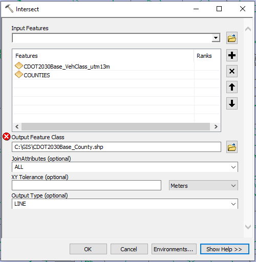
The resulting output feature class had the same geometry and attributes as the TDM shapefile except for the following changes:
- Each link was attributed with the county name and FIPS number.
- Links within multiple counties were split (divided) into separate features at the county line(s). In these cases:
- Both features still had the same attributes except for the county name and FIPS.
- The distance attribute in the “DIST” field was now invalid since the feature was split.
To account for changes in distances for links that were in multiple counties, a new field “cntyMiles” was added to the output feature class. The geoprocessing tool “Calculate Geometry” was used on the “cntyMiles” field to calculate the distance of each link in miles. The “cntyMiles” field, rather than the “DIST” field, was used later in Access to calculate VMT.
The resulting attribute table was saved as a CSV file and used in the following steps.
Access Database
The TDM CSV file from the step above was imported into an Access database. The remaining post-processing steps were performed in this Access database, as described below.
Speeds
The TDM speeds were in floating decimal format and rounded to the nearest integer. Speeds less than 2.75 mph were rounded to 2.5 mph. This was because emission rates for speeds of 2.5 mph or less were the same, as described in the Processed Emission Rates section.
Time Periods
The TDM model provides aggregated data for 10 blocks of time for a day, not hour by hour—see the “name” column below. The data for these TDM periods were recategorized/interpolated into data for discrete clock hours 1-24 based on methodology from APCD.
The PeriodHour24 table below was used to split the TDM data for different time periods (AM1, PM2, OP1, etc.) into 24 clock hour time periods. VMT was calculated for each combination of integer speed (2.5 – 75mph), interstate (yes or no), road functional class (1-8), rural (yes or no), periodCog (1-10), and county.
The periodCog 1-10 were related to hours 1-24 as shown in the “hour” column. That provided a VMT per clock hour for each combination of speed and functional class. This was used to relate the VMT to fractions of VMT by HPMS per functional class and hour.
The cVMT was divided by the number of “periods” corresponding with each clock hour to calculate the VMT.
| Interval | periodCog | name | hour | hrsT | periods |
|---|---|---|---|---|---|
| 11:00 PM – 6:30 AM | 7 | Op1.bin | 1 | 7.5 | 7 |
| 11:00 PM – 6:30 AM | 7 | Op1.bin | 2 | 7.5 | 7 |
| 11:00 PM – 6:30 AM | 7 | Op1.bin | 3 | 7.5 | 7 |
| 11:00 PM – 6:30 AM | 7 | Op1.bin | 4 | 7.5 | 7 |
| 11:00 PM – 6:30 AM | 7 | Op1.bin | 5 | 7.5 | 7 |
| 11:00 PM – 6:30 AM | 7 | Op1.bin | 6 | 15 | 7 |
| 6:30 – 7:00 AM | 1 | Am1.bin | 7 | 1 | 1 |
| 7:00 – 8:00 AM | 2 | Am2.bin | 8 | 1 | 1 |
| 8:00 – 9:00 AM | 3 | Am3.bin | 9 | 1 | 1 |
| 9:00 – 11:30 AM | 8 | Op2.bin | 10 | 2.5 | 2.5 |
| 9:00 – 11:30 AM | 8 | Op2.bin | 11 | 2.5 | 2.5 |
| 9 | Op3.bin | 12 | 3.5 | 7 | |
| 8 | Op2.bin | 12 | 2.5 | 5 | |
| 11:30 AM – 3:00 PM | 9 | Op3.bin | 13 | 3.5 | 3.5 |
| 9 | Op3.bin | 14 | 3.5 | 3.5 | |
| 9 | Op3.bin | 15 | 3.5 | 3.5 | |
| 3:00 – 5:00 PM | 4 | Pm1.bin | 16 | 2 | 2 |
| 3:00 – 5:00 PM | 4 | Pm1.bin | 17 | 2 | 2 |
| 3:00 – 6:00 PM | 5 | Pm2.bin | 18 | 1 | 1 |
| 6:00 – 7:00 PM | 6 | Pm3.bin | 19 | 1 | 1 |
| 7:00 – 11:00 PM | 10 | Op4.bin | 20 | 4 | 4 |
| 7:00 – 11:00 PM | 10 | Op4.bin | 21 | 4 | 4 |
| 7:00 – 11:00 PM | 10 | Op4.bin | 22 | 4 | 4 |
| 7:00 – 11:00 PM | 10 | Op4.bin | 23 | 4 | 4 |
| 11:00 PM – 6:30 AM | 7 | Op1.bin | 24 | 7.5 | 7 |
Fraction of VMT by HPMS
Once VMT was calculated for each road functional class and clock hour, the fractions of VMT by HPMS for each corresponding functional class and clock hour were applied. This calculated the VMT for HPMS 10-60. The fractions used were from APCD and were consistent with their methodology.
| NAA? | Weld? | Rural? | FC | Hr | 10f | 20f | 30f | 40f | 50f | 60f |
|---|---|---|---|---|---|---|---|---|---|---|
| -1 | W | R | 1 | 1 | 1.12494375281236E-03 | 0.442984079764564 | 0.442981870287873 | 8.24958752062397E-04 | 3.60606876834793E-03 | 0.14247807867434 |
| -1 | W | R | 1 | 2 | 6.50325162581291E-04 | 0.418107821883677 | 0.388118179039889 | 1.40070035017509E-03 | 5.57032759041272E-03 | 0.186152645973265 |
| -1 | W | R | 1 | 3 | 1.1907462009526E-03 | 0.402448608970853 | 0.376594285267901 | 1.9278748015423E-03 | 8.86488378110699E-03 | 0.208973600977645 |
| -1 | W | R | 1 | 4 | 1.88772529102432E-03 | 0.400795540811441 | 0.375296865809669 | 3.5956672209987E-03 | 8.74568726325532E-03 | 0.209678513603612 |
| -1 | W | R | 1 | 5 | 1.27600843728028E-03 | 0.438002933384539 | 0.406922735865401 | 8.59352621025494E-04 | 5.91653137282429E-03 | 0.14702243831893 |
| -1 | W | R | 1 | 6 | 9.86892049192773E-04 | 0.462978652961131 | 0.429325812630245 | 1.88521686320158E-03 | 5.20852159466524E-03 | 9.96149039015637E-02 |
| -1 | W | R | 1 | 7 | 8.56477631797771E-04 | 0.47063947538398 | 0.437825973989187 | 1.19740562115417E-03 | 7.50554404406707E-03 | 8.19751233298142E-02 |
Road Types
The TDM used roadway functional classes that were recategorized to MOVES road types. That allowed the road types from the TDM to be related to the emission rates.
| DRCOG Facility | FHWA Facility Type | rural? | FHWA | Urban | MOVESrt | fhwaRT | fcCode | Interstate |
|---|---|---|---|---|---|---|---|---|
| 1 | Principal Arterial – Interstate | -1 | R | R | 2 | 1 | 1 | 1 |
| 1 | Principal Arterial – Interstate | -1 | R | R | 2 | 1 | 1 | 0 |
| 1 | Principal Arterial – Interstate | 0 | N | U | 4 | 11 | 1 | 0 |
| 1 | Principal Arterial – Interstate | 0 | N | U | 4 | 11 | 1 | 1 |
| 2 | Principal Arterial – Other | -1 | N | R | 3 | 2 | 2 | 0 |
| 2 | Principal Arterial – Other Freeways or Expressways | 0 | N | U | 4 | 12 | 2 | 0 |
| 3 | Principal Arterial – Other | -1 | N | R | 3 | 2 | 3 | 0 |
| 3 | Principal Arterial – Other | 0 | N | U | 5 | 14 | 3 | 0 |
| 4 | Minor Arterial | -1 | N | R | 3 | 6 | 4 | 0 |
| 4 | Minor Arterial | 0 | N | U | 5 | 16 | 4 | 0 |
| 5 | Major Collector | -1 | N | R | 3 | 7 | 5 | 0 |
| 5 | Collector | 0 | N | U | 5 | 17 | 5 | 0 |
| 6 | Principal Arterial | -1 | R | R | 2 | 1 | 1 | 0 |
| 6 | Principal Arterial | 0 | N | U | 4 | 11 | 1 | 0 |
| 8 | Local System | -1 | N | R | 3 | 9 | 7 | 0 |
| 8 | Local System | 0 | N | U | 5 | 19 | 7 | 0 |
Filter by Geography/Region
The statewide GHG inventory was filtered to contain VMT for all counties in Colorado except for the nine-county region in the ozone non-attainment area. The nine counties excluded were Adams, Arapahoe, Boulder, Broomfield, Denver, Douglas, Jefferson, Larimer, and Weld. The statewide results were subdivided further into Pikes Peak area and the rest of the state.
Emissions Inventory
The processed emission rates table and the processed VMT table were related by road type, HPMS type, hour, and speed. This relate was used to multiply the emission rate (g/mi) by the VMT (mi) to get a total in grams of CO2e for an average weekday. The formula used was:
- CO2e (g/day) = SUM(Emission Rate (g/mi) * VMT (mi))
- CO2e (MMt/day) = CO2e (g/day) * 1 (MMt) / 1e+12 (g)
- CO2e (MMt/year) = CO2e (MMt/day) * 338 (TDM weekdays/calendar year)
The calculated emissions inventory was for on-road emissions. Non-road emissions were not included in this calculation.
References
EPA. 2016. Using MOVES for Estimating State and Local Inventories of On-road Greenhouse Gas Emissions and Energy Consumption. June. https://nepis.epa.gov/Exe/ZyPDF.cgi?Dockey=P100OW0B.pdf