Appendix E: Greenhouse Gas Transportation Report – Calibration and Validation Report

5.2 TDM Calibrations and Validation Report

Pikes Peak Travel Demand Model Update

PTV Group in cooperation with the Pikes Peak Area Council of Governments updated the multimodal tour-based travel demand model that represents travel activity in the region. This model update also enhanced the model with the addition of a work from home variable in the tour generation step and a 24hr dynamic traffic assignment model. The dynamic assignment model is a regional scale mesoscopic traffic simulation with more than 700 signalized intersections. The base year for the model is set to 2020.

This transportation planning model is a tour-based model and is a representation of the Colorado Springs area transportation facilities and multimodal travel patterns using these facilities. The model contains inventories of the existing roadway facilities, transit lines, synthetically generation population at the household and person level, as well as land use data such as workers, student enrollment, shopping, employment etc. in the area. The travel demand model was calibrated to reflect average daily traffic on roadway facilities. Further, hourly traffic counts were used to calibrate hourly travel demand for the purpose of dynamic traffic assignment.

The model can be used to measure the impact and evaluate scenarios such as changes in population, employment centers, travel behavior patterns, or roadway improvements. The transportation engineer or planner, using the transportation planning model, can project future traffic volumes without the cost of building inappropriate roadways or waiting for traffic congestion to severely impact travelers.

The model was developed using VISUM 2024. VISUM is a Windows based multimodal transportation modeling software and has an array of features implemented in an easy-to-use graphical user interface, thereby making it a very powerful analysis tool for transportation modeling and planning.

This document details the methodology that was used to develop the model. Because modeling is a complex process, much of the theory, terminology, and concepts are also discussed.

1. Model Area Identification

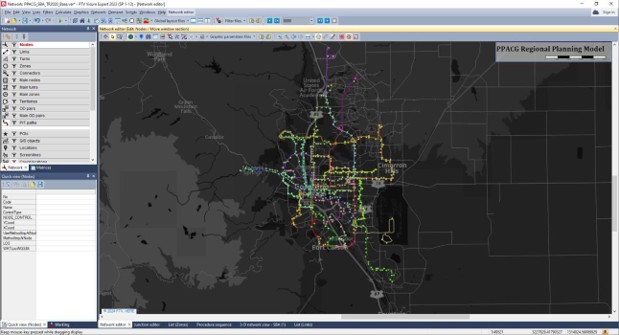
The model area contains El Paso County, Colorado Springs, Manitou Springs, Woodland Park, Green Mountain Falls, Fountain, Palmer Lake and Monument. The major through route in the area is I-25. The route runs in a north-south direction, with Denver in the north and Pueblo in the south. A snapshot of the model area is shown in Figure 1.

Figure 1: Travel Demand Model Area – Pikes Peak Area Model

2. Network Development

The updated model network is multi-resolution in structure. Here, the level of detail used in the network assignments can be increased or decreased based on the network assignment method. The static assignment uses a typical link-node structure and applies turn prohibitions and macroscopic volume delay functions to model volume-based network delay. The simulation-based assignment (SBA) uses intersection geometry details and intersection control including signal timings and stop/yield control.

Network development for the model involved the following items:

1. Street network development – lanes, speeds, intersection geometries, signal timings etc.
2. Transit network development – transit lines with related timetable and headway data.
3. Transportation analysis zone refinement and updated centroid connectors.

2.1 Street Network Development

The street network for the model was developed by refinement of the existing travel demand model network using GIS layers and aerial imagery. The roadway classes, speeds, capacities and number of lanes were checked and updated in the entire network. In addition, intersection control, geometry and signal timings were added to the network to represent intersection level delay more accurately for the purpose of dynamic traffic assignment.

The following roadway functional classifications were used for modeling link delays in the model:

Table 1: Model and Link Classification

Type No	Class No	Class Name	Capacity (/hr/ln)	Speed	Delay Function
10	1	Interstate HOV Connection	1500	65	1
11	1	Interstate	2400	80	1
12	1	Interstate	2400	75	1
13	1	Interstate	2400	70	1
14	1	Interstate	2350	65	1
15	1	Interstate	2300	60	1
16	1	Interstate	2250	55	2
17	1	Interstate HOV	1500	75	1
18	1	Interstate HOV	1500	70	1
19	1	Interstate HOV	1500	65	2
20	2	Expressway	2000	65	3
21	2	Expressway	2000	60	3
22	2	Expressway	1850	55	4
23	2	Expressway	1700	50	4
24	2	Expressway	1550	45	4
25	2	Expressway	1500	40	5
26	2	Expressway	1450	35	8
27	2	Expressway	1400	30	9
28	2	Expressway	1350	25	10
29	2	Expressway	1850	70	1
30	3	Principal Arterial	1800	65	4
31	3	Principal Arterial	1800	60	4
32	3	Principal Arterial	1800	55	5
33	3	Principal Arterial	1200	50	5
34	3	Principal Arterial	1000	45	6
35	3	Principal Arterial	900	40	7
36	3	Principal Arterial	850	35	8
37	3	Principal Arterial	800	30	9
38	3	Principal Arterial	800	25	10
40	4	Minor Arterial	1000	55	4
41	4	Minor Arterial	1000	50	5
42	4	Minor Arterial	850	45	6
43	4	Minor Arterial	850	40	7
44	4	Minor Arterial	750	35	8
45	4	Minor Arterial	700	30	9
46	4	Minor Arterial	700	25	10
47	4	Minor Arterial	650	20	10
48	4	Minor Arterial	650	15	10
49	4	Minor Arterial	1000	65	1
50	5	Collector	850	55	5
51	5	Collector	850	50	5
52	5	Collector	650	45	6
53	5	Collector	650	40	7
54	5	Collector	650	35	8
55	5	Collector	650	30	9
56	5	Collector	650	25	10
57	5	Collector	600	20	11
58	5	Collector	600	15	11
59	5	Collector	600	10	11
60	6	Residential	600	35	8
61	6	Residential	600	30	9
62	6	Residential	550	25	10
63	6	Residential	550	20	11
70	7	Ramp	1250	60	3
71	7	Ramp	1200	55	4
72	7	Ramp	1200	50	5
73	7	Ramp	1200	45	6
74	7	Ramp	1200	40	7
75	7	Ramp	1200	35	8
76	7	Ramp	1000	30	9
77	7	Ramp	1000	25	10
78	7	Ramp	1000	20	11
79	7	Ramp	1000	15	12

The above link capacities were applied in the network in combination with BPR volume delay functions to capture volume to capacity-based delay. The functional form is shown in the Figure 2 below.

Figure 2: Link Volume Delay Function for the PPACG Model

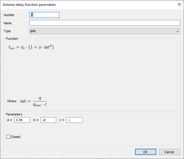
Six parameter sets were used in the model. These are shown in the table below:

Table 2: BPR Volume Delay Function Parameters

Delay Function No	BPR_a	BPR_b
1	0.98	10.0
2	0.93	8.0
3	1.00	5.4
4	0.83	2.7
5	0.71	2.1
6	0.15	7.0
7	0.15	7.0
8	0.15	7.0
9	0.15	7.0
10	0.15	7.0
11	0.15	7.0
12	0.15	7.0
13	0.15	7.0

2.2 Transit Network Development

The PPACG tour-based model is designed as a 24-hour model with user defined time of day outputs. As a result, the network from the previous version of the model was completely replaced with a high-resolution transit network based on General Transit Feed Specification (GTFS). This network contains detailed timetable information suitable for timetable-based assignment and other operational analyses related to transit. While the existing model does not use timetable-based transit assignment, storing a timetable allows calculation of transit isochrones by time of day. This is useful in obtaining more realistic measures of transit accessibility and timed transfer connections at a disaggregated level.

A summary of transit lines included in the base model is presented in the table below.

Table 3: Base Model Transit Lines

Line Name	Route ID	Route Name	TSYS Name
MMT_3416	1	Hillside – Hancock Plaza	Bus
MMT_3417	10	Hwy 115 – PPSC	Bus
MMT_3418	11	World Arena – PPSC	Bus
MMT_3419	12	Palmer Park Blvd	Bus
MMT_3420	14	Chestnut St – G.O.G. Rd	Bus
MMT_3421	15	Fountain Blvd – E Cheyenne Mtn Blvd	Bus
MMT_3422	16	Brookside – Uintah Gardens	Bus
MMT_3423	17	19th Street / Fillmore	Bus
MMT_3424	18	Union Blvd	Bus
MMT_3425	19	Weber – Eagle Rock	Bus
MMT_3426	2	Centennial Blvd – G.O.G. Rd	Bus
MMT_3427	22	Southborough via Murray Blvd	Bus
MMT_3428	23	Barnes Rd. – Tutt Blvd	Bus
MMT_3429	24	Galley Rd – Tutt Blvd	Bus
MMT_3430	25	N. Academy Blvd – Voyager	Bus
MMT_3431	27	S. Academy Blvd – PPSC	Bus
MMT_3432	3	Colorado Ave – Manitou	Bus
MMT_3433	32	Security / Widefield	Bus
MMT_3434	33	Incline / Cog Shuttle	Bus
MMT_3435	34	G.O.G. / Austin Bluffs Pkwy	Bus
MMT_3436	35	Las Vegas St / PPSC	Bus
MMT_3438	37	Amazon / Airport	Bus
MMT_3439	38	Union / Children’s Hospital	Bus
MMT_3440	39	Corporate Dr / Voyager Pkwy	Bus
MMT_3441	4	S. 8th Street – Broadmoor	Bus
MMT_3442	40	Voyager – Rampart PPSC	Bus
MMT_3443	5	Boulder – Citadel	Bus
MMT_3444	6	Fillmore – Citadel	Bus
MMT_3445	7	Pikes Peak Ave. – Citadel	Bus
MMT_3446	8	Cache La Poudre – Citadel	Bus
MMT_3447	9	Nevada – UCCS	Bus
MMT_3448	ZEB	ZEB Downtown Shuttle	Bus

Figure 3: GTFS Based Transit Network for the PPACG Model

2.3 Transportation Analysis Zone Refinement

The original TAZ system for the PPACG model was reviewed and revised to better align with census boundaries and roadway infrastructure. The updated TAZ system consists of 945 zones out of which 11 zones are external stations. The traffic and transit loading points or connectors were also redefined and placed as appropriate. The same loading scheme is used in both static and dynamic network assignments. The updated TAZ system for the PPACG Tour Based Model is illustrated below.

Figure 4: Updated TAZ System for the PPACG Model

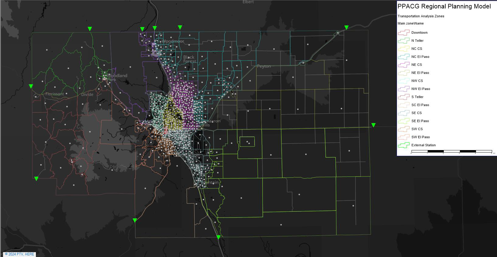
Table 4: PPACG TAZ System Summary

District	Number of Zones
Downtown	72
N Teller	19
NC CS	100
NC El Paso	129
NE CS	182
NE El Paso	14
NW CS	79
NW El Paso	22
S Teller	26
SC El Paso	8
SE CS	183
SE El Paso	23
SW CS	62
SW El Paso	15
External Station	11
TOTAL	945

2.4 Land Use Data

The land use and demographic data for the tour-based model was developed from multiple sources. The MPO provided the population and employment cross-sections. Additionally, the land use data related to zone level employment, shopping, recreation and student enrollment was derived from GIS data maintained by the MPO.

2.5 Demographic Data – Population Synthesis

The PPACG model uses a disaggregate synthetic population. The population synthesis process generates household weights for the seed sample that satisfies the marginal distributions. The final weights are then used to expand the seed sample into a disaggregate synthetic population. The use of a synthetic population allows greater flexibility in modeling tour and trip making characteristics by various demographic cross-sections and incorporation of variables to model work-from-home situations in a more robust and flexible manner.

With the advancement of travel demand models in recent years, synthetic population generation has also received research attention. Traditional population synthesizers used Iterative Proportional Fitting (IPF) or Iterative Proportional Updating (IPU) methods while advanced population synthesizers use optimization-based techniques such as entropy maximization and linear programming. PopulationSim¹ is a state-of-the-art population synthesizer software originally developed for the Oregon Department of Transportation (ODOT) and its partner agencies. PopulationSim is an open software developed in the ActivitySim² framework and is currently managed by the ActivitySim consortium. PopulationSim offers many technical and usability enhancements over other population synthesizers.

PopulationSim makes several advancements over traditional population synthesizers such as PopSyn3 and PopGen. These include enhancements resulting from the use of advanced optimization methods, unique features for travel demand model applications, efficient software design, and better interfacing with PTV Visum. The following sub-sections describe these benefits in more detail.

Algorithmic Advantages

PopulationSim uses an entropy maximization-based list-balancing approach for generating weights³. The entropy-maximization formulation results in uniform weights that are not expanded beyond a user-defined threshold. The uniformity in weights ensures that the distribution of uncontrolled variables is not significantly changed in the process. This unique formulation also allows for the specification of importance factors on each marginal control. The user can set these factors in accordance with their confidence in the quality of the data.

Another important advantage of the PopulationSim algorithm is that it operates simultaneously on all geographic units. This eliminates the errors resulting from the sequential processing of geographies. This is a known problem in the PopSyn3 population synthesizer which results in poor control match for minority population segments such as university students or low-income households. The simultaneous list balancing method used in PopulationSim eliminates this type of error and results in better control match for minority population segments.

Generally, the list balancing or IPF-based process generates floating-point weights. However, for expanding the seed sample, integer weights are required. Many traditional population synthesizers resort to simple or bucket rounding of floating-point weights. This method results in poor control matches and the errors can accumulate over geographic units. Some IPF-based population synthesizers such as PopGen rely on Monte-Carlo draws from a joint distribution of floating-point weights. Again, the Monte-Carlo errors can accumulate and result in poor marginal control matches. PopulationSim uses a linear programming (LP) formulation to convert floating-point weights to integers. As a result, PopulationSim avoids rounding or drawing errors in contrast to other population synthesizers.

Advanced Usability Features

PopulationSim also offers several unique features that make it a practical choice for many travel demand model applications. These features are described below:

Person Controls

PopulationSim allows the specification of both household and person-level controls. While most population synthesizers offer this feature, some of the traditional ones operate only at the household level.

Multiple Geographies

As stated earlier, the main inputs to the population synthesis process are a seed sample and marginal controls. Typically, most population synthesizers operate at a single geographic level. However, data for marginal controls are generally not available at the same geographic level. For example, the household income distributions may be available at the Traffic Analysis Zone (TAZ) level and the person age distribution might be available at the County level. The available data needs to be transformed to the same geographic level which can be a time-consuming task and can introduce approximation errors. In contrast, PopulationSim can use data available at multiple geographic levels without any transformation.

Importance Factors for Controls

As stated earlier, PopulationSim also allows users to specify importance factors on each control. The PopulationSim algorithm gives higher priority to marginal controls with a higher importance factor. This feature can be very useful in a situation where the user places a higher level of confidence in a certain data source.

Re-populate Feature

Typical model applications for a regional model include corridor studies and traffic impact studies, which require carefully controlled baseline versus build analysis. PopulationSim software offers functionality that supports this type of analysis; a ‘re-populate’ mode in the software adds to or replaces the existing synthetic population in a subset of zones using whatever controls the user is able to provide (for example, households by type).

Software Benefits

As mentioned earlier, PopulationSim has a robust open-source software implementation in the ActivitySim framework. Software development adheres to software engineering best practices. The system is under continuous integration (CI), which means the software and documentation are automatically built and tested against sample datasets to ensure that new features do not break the code base for any users. PopulationSim benefits arising from its robust software design are described below:

Runtime

The Python-based ActivitySim framework makes heavy use of the Numpy and Pandas Python libraries, which allow for the vectorization of operations to reduce overall runtime. This in conjunction with an optimization-based algorithm achieves faster convergence for PopulationSim. Runtime comparison between PopGen and PopulationSim for DVRPC and NFTPO showed significant runtime improvements.

ActivitySim Framework

The software depends on the ActivitySim core and therefore offers the same user experience as the ActivitySim activity-based model, namely the same user interface, customizable expressions, approach to tracing calculations, and data management.

Documentation and Support

The PopulationSim source code and technical documentation are available at the following public GitHub repository: https://github.com/ActivitySim/populationsim. The technical documentation includes runnable examples and training resources. PopulationSim enjoys a large user community in the US and worldwide. The users can report bugs and issues on the GitHub repository and contribute to the software development.

Integration with PTV Visum

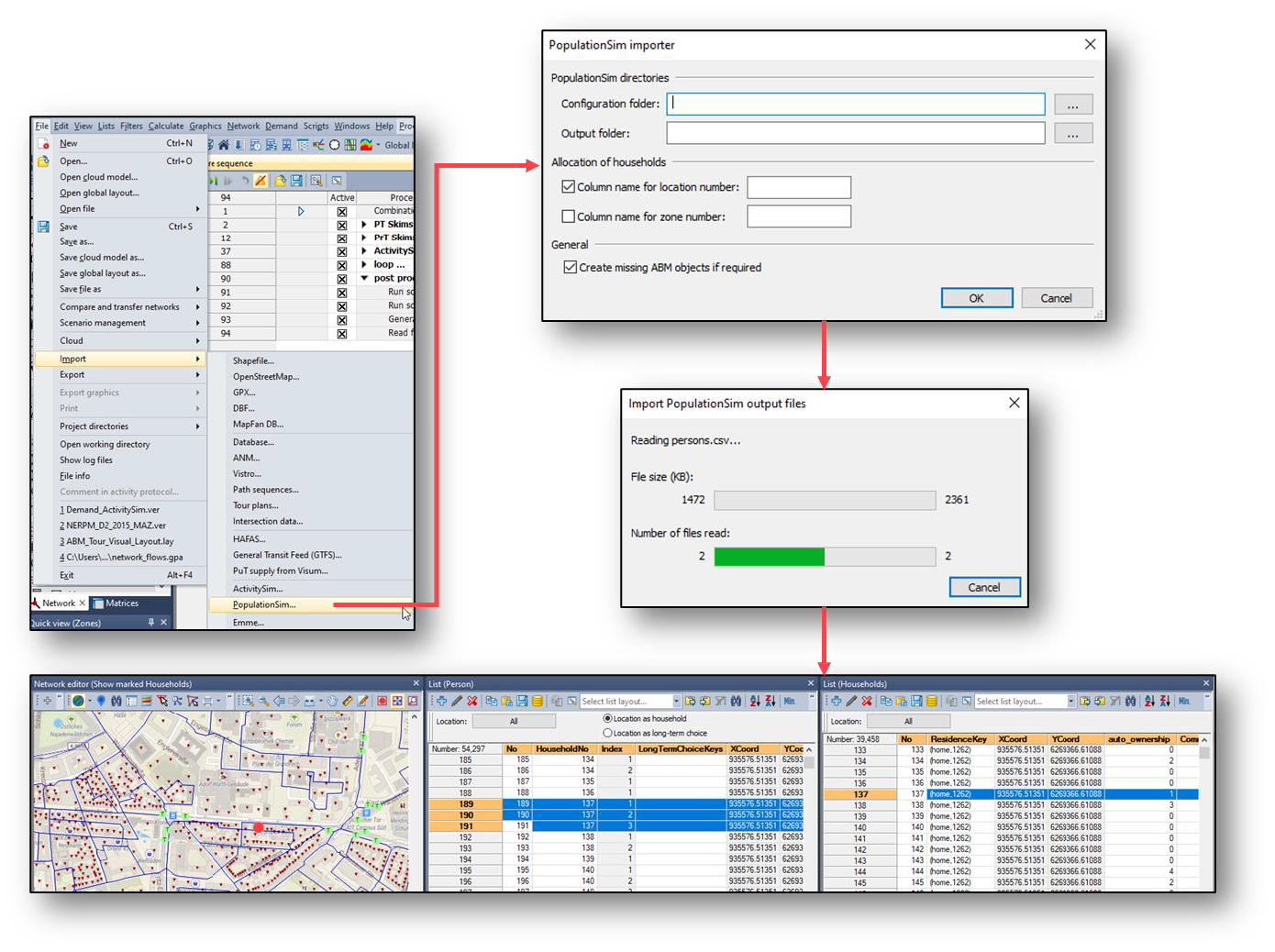
Visum now includes person and household Network Objects to house synthetic populations. Visum’s Python API or the GUI-based menu option can be used to import PopulationSim-generated synthetic population. The user points Visum to an existing PopulationSim setup. The import procedure reads the outputs into Visum and creates network objects as needed.

Figure 5: PTV Visum PopulationSim Import Procedure

The list of land use and demographic variables used in the model is given in the Appendix.

3. Model Approach

The tour-based model structure adopted in Visum is based on a hybrid modeling methodology which explicitly models person tour generation at the individual level and combined mode-destination and time of day choice of homogeneously divided person types at an aggregated zonal level. It involves execution of the following procedures:

1. Tour generation
2. Tour destination choice – with and without rubber banding
3. Tour mode choice – with primary mode choice or leg-by-leg mode choice
4. Time of day calculation – based on trip level time of day factors derived from survey data

The three logical units (mode-destination-time of day choice) are processed simultaneously during the model calculation.

Figure 6: PPACG Tour Based Model Calculation Flow

3.1 Tour Generation

Tour generation (calculating and applying skeletal tour/activity patterns by person type): In the hybrid modeling approach, tour generation is calculated at the person level using a range of person and household attributes. Subsequently, the person level results are aggregated into a set of broader person groups which are used to summarize model results and application of mode-destination and time of day models.

Table 5: PPACG Model Person Groups

Code	Name
Worker_GCP	General, Clerical and Professional Workers
Worker_MCT	Manufacturing, Construction and Trades Workers
Worker_MIL	Military Workers
NonWorker	Non-Workers under 65
Senior	Non-Workers 65 and above
Student_Elem	Student Elementary School
Student_High	Student High School
Student_Univ	Student College University

The updated tour generation model incorporates a work-from-home model to accommodate the impact of new work-from-home trends seen after the COVID19 pandemic. The approach used in the PPACG tour generation model to account for work-from-home policies is applied as a post-processing step in tour generation that scales the base tour generation to produce updated tour frequencies for each worker in the synthetic population.

In the first step, a mobility rate is calculated for each person and tour type combination. To calculate mobility rates, daily activity chains derived from a travel survey are broken down into individual home-based tours. Distinct tour types are identified among the complete set of tours and their corresponding probability is calculated. As a result, the sum of the probabilities of a person group can be greater than 1.0 (or 100 %), because a person can execute multiple tours one after the other in a day (for example: first HWH, then HOH).

Consider for example the daily activity chains 5 persons below:

HWH, HWH, HWOH, HWHOH, HOHWH

In the above case, mobility rates for home-based tours (HWH, HWOH, HOH) tours are calculated by counting their occurrence in each of the daily activity chains and dividing it by the total number of daily activity chains.

This produces a mobility rate of 0.8 [4/5] for HWH, a mobility rate of 0.4 [2/5] for HOH and a mobility rate of 0.2 [1/5] for HWOH tours.

Mobility rate extraction from the travel diary coarsely involves the steps below,

1. Extraction of raw chains or daily patterns for each person type
2. Determining unique home-based tours within the chains
3. Counting the occurrence of each tour type in the list of all chains and dividing by the number of activity chains.

The base mobility rates for each person group and tour type derived from the PPACG travel survey are tabulated below. Activities in the tour chain are represented as: H-Home, W-Work, D-Stop on work/school, O-Non-work.

No	Tour	Worker GCP	Worker MCT	Worker MIL	Non-Worker	Senior	Student Elem	Student High	Student Univ
1	HDDDWDD DH	0	0	0	0	0	0	0	0
2	HDDDWDD H	0	0	0	0	0	0	0	0
3	HDDDWDH	0	0	0	0	0	0	0	0
4	HDDDWH	0.01	0.01	0	0	0	0	0	0
5	HDDSDDH	0	0	0	0	0	0	0.01	0.01
6	HDDSDH	0	0	0	0	0	0	0	0
7	HDDSH	0	0	0	0	0	0	0	0
8	HDDWDDD H	0	0.01	0	0	0	0	0	0
9	HDDWDDH	0	0	0	0	0	0	0	0
10	HDDWDH	0.01	0.01	0	0	0	0	0	0
11	HDDWH	0.01	0	0.01	0	0	0	0	0
12	HDSDDH	0	0	0	0	0	0.01	0	0.01
13	HDSDH	0	0	0	0	0	0.05	0.05	0.01
14	HDSH	0	0	0	0	0	0.03	0.06	0.01
15	HDWDDDH	0.02	0.02	0.02	0	0	0	0	0
16	HDWDDH	0.02	0.01	0.02	0	0	0	0	0
17	HDWDH	0.03	0.01	0.06	0	0	0	0	0
18	HDWH	0.05	0.03	0.04	0	0	0	0	0
19	HOH	0.44	0.41	0.25	0.67	0.55	0.38	0.26	0.44
20	HOOH	0.16	0.12	0.09	0.26	0.22	0.12	0.05	0.15
21	HOOOH	0.07	0.04	0.03	0.1	0.06	0.04	0.05	0.06
22	HOOOOH	0.09	0.06	0.01	0.11	0.11	0.04	0.03	0.07
23	HSDDH	0	0	0	0	0	0.04	0.1	0.04
24	HSDH	0	0	0	0	0	0.08	0.12	0.03
25	HSH	0	0	0	0	0	0.42	0.5	0.22
26	HWDDDH	0.06	0.05	0.02	0	0	0	0	0
27	HWDDH	0.05	0.05	0.06	0	0	0	0	0
28	HWDH	0.08	0.07	0.07	0	0	0	0	0
29	HWH	0.4	0.5	0.5	0	0	0	0	0

In the second step, a person level work from home multinomial choice model is used to estimate the probability of a person working from home for a given number of days. This provides a scaling factor that is then applied to the ‘base’ work tour mobility rate for each person. The model coefficients for the telecommute frequency choice model were initially adopted from the SANDAG travel demand model and calibrated to the available remote-work data available in the travel survey. The coefficients adopted in the model are tabulated below.

Table 7: Remote Work Choice Model Parameters

		Telecommute Alternative Coefficients
No	Variable	no_telecommute	1_day_week	2_3_day_week	4_days_week
1	occp_Services	0	-1.62	-0.65	0
2	occp_SalesOffice	0	-0.62	-0.74	-0.89
3	occp_ResourceConstruct	0	-1.57	0	0
4	occp_TransportMat	0	-14.75	0	0
5	presenceOfChildren0_5	0	0	0	-0.86
6	presenceOfChildren6_12	0	0	0.52	-0.81
7	adultInHousehold_1	0	0.18	0	-0.04
8	adultInHousehold_ge2	0	0	0	0
9	female	0	0	0	0
10	partTimeWorker	0	0	0.42	1.11
11	univStudent	0	0	0.6	0
12	paysToPark	0	0.46	0	0
13	income_60_100k	0	0.56	0.39	0
14	income_100_150k	0	0.64	0.19	0
15	income_150k_pl	0	0.92	0.77	0
16	autos_0	0	0	0.41	0
17	autos_1	0	0	0	0
18	autos_ge3	0	0	-0.73	0
19	avgDistToWork	0	0.02	0	0
20	ASC	0	-3.62	-3.55	-4.57
21	CALIB_CONST	0	0.57	0.77	1.65

The framework above allows a flexible way to account for the impact of remote work policies on work related travel. This flexibility in the model is necessary because the remote work policies of employers are still evolving post-pandemic (COVID19). The tour generation mode considers that certain types of workers may not be able to work remotely due to the nature of their job (military, manufacturing, service). The models are thus applied based on workers classified by occupation types rather than income. The summaries for the base model are shown below.

Figure 7: Telecommute Model Validation

Observed		Estimated		Estimated Scaled		Observed %		Estimated %
TelecommuteFreq	Workers	TelecommuteFreq	Workers	TelecommuteFreq	Workers	TelecommuteFreq	Percent	TelecommuteFreq	Percent
1_day_week	16,052	1_day_week	18,899	1_day_week	18,899	1_day_week	6.3%	1_day_week	5.9%
2_3_days_week	16,903	2_3_days_week	19,344	2_3_days_week	19,344	2_3_days_week	6.7%	2_3_days_week	6.1%
4_days_week	14,198	4_days_week	14,270	4_days_week	14,270	4_days_week	5.6%	4_days_week	4.5%
no_telecommute	206,952	no_telecommute	266,628	no_telecommute	266,628	no_telecommute	81.4%	no_telecommute	83.%
Total	254,104	Total	319,141	Total	319,141	Total	100%	Total	100%

Table 8: Summary of Base Year Person Tours

Person Group	Persons	Work / School Tours	Other Tours	Total Tours
Worker_GCP	257,151	179,257	204,696	383,952
Worker_MCT	59,428	42,727	39,103	81,829
Worker_MIL	22,093	16,766	8,825	25,591
NonWorker	112,822	–	129,559	129,559
Senior	92,989	–	88,154	88,154
Student_Elem	143,255	91,617	84,293	175,910
Student_High	47,740	40,155	18,552	58,706
Student_Univ	47,864	15,679	34,857	50,536

3.2 Tour Based Destination and Mode Choice

Destination choice/trip distribution (determining the trip destination): The hybrid approach used in the PPACG model implements the tour-based destination choice at a zonal aggregate level. Modeling of

tours considers non-home-based trips as part of a trip chain. This makes the non-home-based trips spatially consistent with the overall trip making in the system. Aggregate tour or trip chain calculations are implemented with matrix operations in a multi-threaded optimized framework. This removes the burden of complicated matrix management from the modeler. Instead, outputs can be specified by time of day and with a flexible combination of activities and modes.

Figure 8: Tour-based Destination-Mode Choice Output Specification

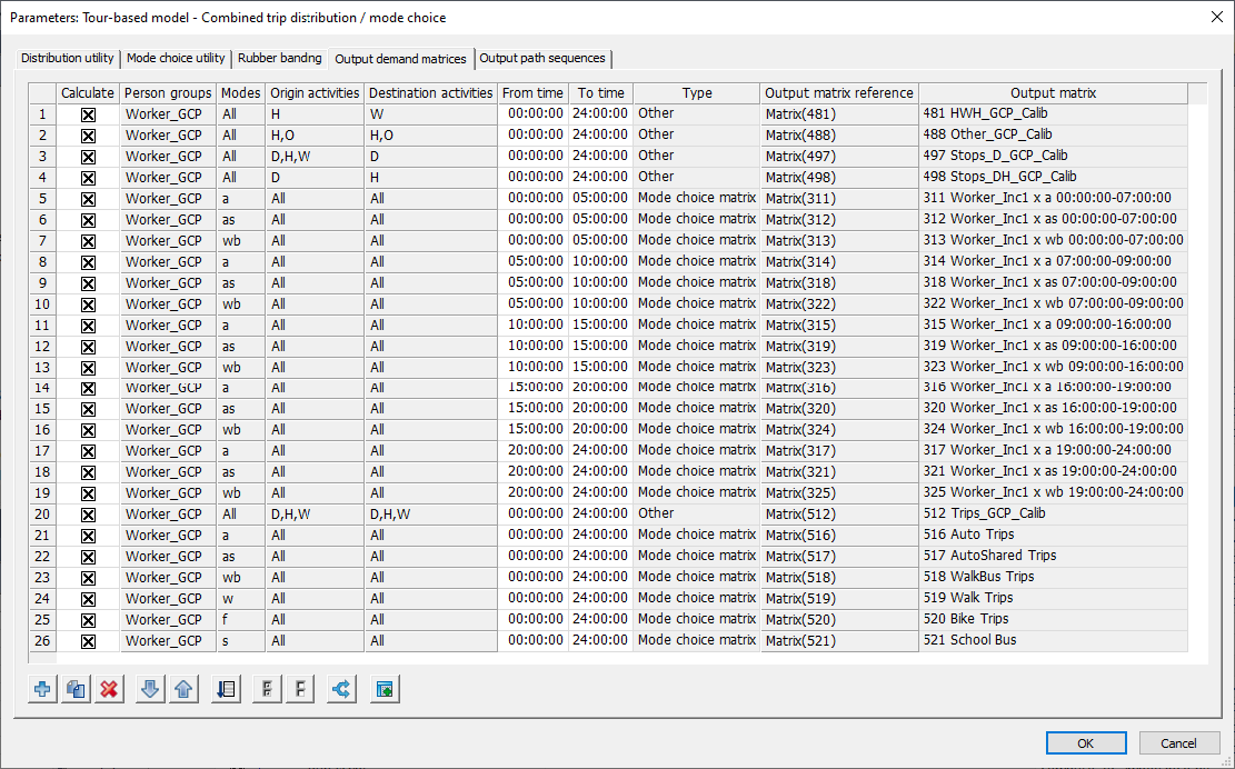
The trip chaining within the tours is calculated in two modes – without rubber-banding (full-tours) and with rubber-banding (half-tours). The methodology for trip chain calculation is described in the next subsections.

Figure 9: Example Tour Types

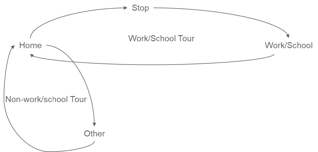
Tours without Primary Activities

The tour-based destination choice is performed using the gravity/destination choice formulation shown below:

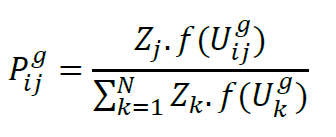
Where,

If f(Uij) is used with a logit function, the above equation becomes equivalent to:

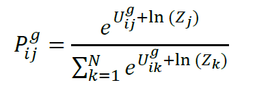
Multiplying out the total number of tours with the above probabilities yields the number of trips along the tour leg. Each trip leg of the home-based tour is evaluated by successively applying the above formulation with each destination leg serving as the origin control for the next leg. As an example, a tour with the skeletal structure HOOH, will be calculated as a chain of matrix operations applied to each leg: HO-> OO->OH. The tour generation provides the initial control trip total for the first trip leg.

Tours with Primary Work/School Activities

Work and school tours are modeled using the concept of rubber-banding. Here, a primary destination governs the choice of mode as well as intermediate stop locations on work and school tours. Consider a tour with skeletal structure HSWH (Home-Stop-Work-Home). Since the primary activity in this tour is

Work (W), the chain is split into two half-tours: (1) HSW and (2) WH. The first half-tour HSW is calculated using the attraction size of the work activity as HW. The trips between H and W are then routed through potential stop locations by using the composite utility of the stop attraction size and friction factor of stop locations with respect to the two anchor locations (Home and Work).

Figure 10: Half Tour with Primary Work Destination and Intermediate Stop Location

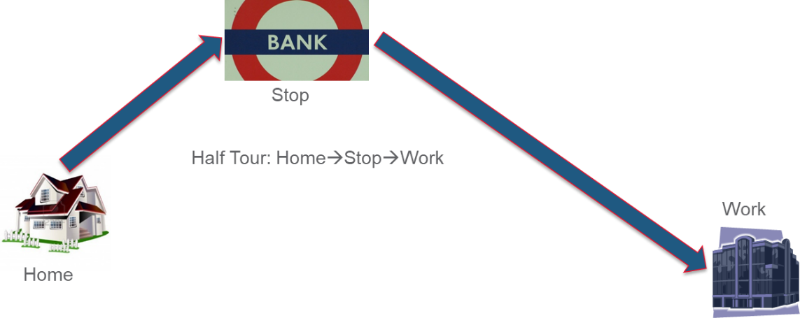
A general consideration for the insertion of stop locations on primary tours is to minimize out of way travel between the primary activity locations (Home and Work/School). The stop location choice is thus based on the composite utility of the trip legs between the primary anchor locations and stop locations. The formulation for intermediate stop location choice is illustrated below:

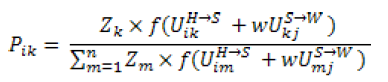
Where,

i = index of origin (home anchor)

j = index of primary destination (work/school)

k = index of intermediate stop location

Zk = size of variable for stop location k

ƒ = functional transformation │ exp

U(HS),(SW) – utilities of traveling to destination through a given stop location

w = weight factor

Destination Choice Model Parameters

The activities considered in the PPACG model are tabulated below:

Activity Name	Activity Code	Anchor Activity
Stop on primary	D	No
Home	H	Yes
Other (Shop/Recreation/Non-work)	O	No
School	S	No
Work	W	No

The size variables used in the model are applied to each person group as a weighted sum of land use variables. The initial set of these weights were based on the SANDAG activity-based model. The weights were then systematically calibrated for the PPACG model to reflect local conditions.

		Land Use Variable
Person Type	Activity	EMP OFFICE	EMP RETAIL	EMP SRVC	EMP LABOR	EMP MIL	HH	EM ENROLL	HS ENROLL	COLL ENROLL	EMP SRVC	EMP RETAIL	EMP OFFICE	EMP SRVC
Senior/Non -Worker	Other	0	0.95	0.3	0	0	0.07	0	0	0	-0.25	-0.8	0	-0.25
Students	Other	0	0.95	0.3	0	0	0.07	0	0	0	-0.25	-0.85	0	-0.25
Workers	Other	0	0.95	0.3	0	0	0.05	0	0	0	-0.25	-0.8	0	-0.25
Elementary	School	0	0	0	0	0	0	1	0	0	0	0	0	0
High	School	0	0	0	0	0	0	0	1	0	0	0	0	0
Post Secondary	School	0	0	0	0	0	0	0	0	1	0	0	0	0
Workers (GCP/MCT)	Stop	0	0.95	0.3	0	0	0.05	0.1	0	0	-0.25	-0.8	0	-0.25
Workers (MIL)	Stop	0	0.95	0.3	0	0	0.05	0.1	0	0	0	0	0	-0.25
Students	Stop	0	0.95	0.25	0.1	0	0.03	0.0 5	0	0	-0.2	-0.85	0	-0.23
Workers (GCP)	Work	0.94	0.83	0.93	0.11	0	0	0	0	0	0	0	0	0
Workers (MCT)	Work	0.06	0.17	0.07	0.89	0	0	0	0	0	0	0	0	0
Workers (MIL)	Work	0	0	0	0	1	0	0	0	0	0	0	0	0

The impedance term in the destination choice model was adopted from the SANDAG model and uses the time, distance and various transformations over destination distance. The coefficients in the model were then systematically calibrated to fit trip length distribution observed from the available travel survey. The impedance related utility coefficients in the model are tabulated below:

Table 9: Impedance Related Utility Coefficients in Destination Choice

Person Type	Activity	Time	Dist	Dist^2	Dist^3	In(Dist +1)
Worker_GCP	Work	-0.04	0.05	0	0	-0.85
Worker_GCP	Other	-0.21	0.04	0	0	-0.75
Worker_GCP	Stop	-1.4	0	0	0	0
Worker_MCT	Work	-0.04	0.05	0	0	-0.85
Worker_MCT	Other	-0.21	0.04	0	0	-0.75
Worker_MCT	Stop	-1.4	0	0	0	0
Worker_MIL	Work	-0.04	0.05	0	0	-0.85
Worker_MIL	Other	-0.21	0.04	0	0	-0.75
Worker_MIL	Stop	-1.4	0	0	0	0
Student_Elem	School	-0.22	-0.07	0	0	-0.9
Student_Elem	Other	-0.21	0.04	0	0	-0.75
Student_Elem	Stop	-1.5	-0.5	-0.03	0	-0.25
Student_High	School	-0.4	-0.15	0	0	0
Student_High	Other	-0.21	0.04	0	0	-0.75
Student_High	Stop	-1.5	-0.5	-0.03	0	-0.25
Student_Univ	School	-0.1	-0.05	0	0	-1.1
Student_Univ	Other	-0.21	0.04	0	0	-0.75
Student_Univ	Stop	-1.5	-0.5	-0.03	0	-0.25
NonWorker	Other	-0.21	0.04	0	0	-0.75
Senior	Other	-0.21	0.04	0	0	-0.75

Destination Choice Model Validation

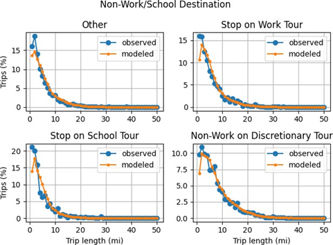
The destination choice models were calibrated for the trip lengths observed in the available household travel survey. A summary of the trip length validation for the modeled primary and secondary trip purposes is given below.

Table 10: Average Trip Length Validation

	Trip Length (miles)
Purpose	HH Survey	Model
Work	8.35	8.85
School (K8)	3.31	3.58
High School	4.26	4.47
Post-Secondary	8.61	8.93
Other/non-work	4.74	5.19
Stops on Work Tour	5.15	5.49
Stops on School Tour	4.17	4.47

Figure 11: Work/School Trip Length Validation

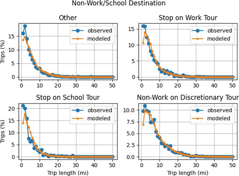
Figure 12: Discretionary and Other Trip Length Validation

Tour Based Mode Choice

Mode choice: The mode choice functional form is the commonly used logit model. Mode choice can be specified at the person type level as well as the destination activity level. In the PPACG model, it is specified at the person type and destination activity level. The freedom of choice restrictions within trip chains where a traveler may switch between travel modes from one leg of the tour to another is accounted for by defining modes as exchangeable or non-exchangeable. Thereafter, the tour-based model calculates a logit choice model. In the tour-based framework, mode choice is computed either based on primary activity when using rubber-banding or applied to each trip leg along the tour when rubber-banding is turned off. Trip chains or tours with work or school were calculated using rubber-banding and other trip chains were calculated using the sequential mode choice model. The coefficients for the mode choice model were adopted from the FHWA-TMIP⁴ guidelines. The constants were then adjusted to align the mode choice results with the available travel survey data.

Six travel modes were considered in the PPACG model. The coefficients and calibrated constants for these are summarized in the tables below.

Table 11: Mode Choice Coefficients

Purpose	Time (Min)	Cost ($)
Work	-0.018	-0.184
Non-work	-0.024	-0.25

Table 12: Calibrated Alternative Specific Constants

Person Type	Purpose	Auto (sov)	Auto (hov)	Transit	Bike	Walk	SchBus
Worker_GCP	Work	0	-3.59	-4.03	-4.04	-3.03	N/A
	Other	0	-1.9	-2.93	-4.04	-2.58	N/A
Worker_MCT	Work	0	-3.59	-5.93	-4.04	-3.03	N/A
	Other	0	-1.9	-4.93	-4.04	-2.58	N/A
Worker_MIL	Work	0	-3.59	-5.93	-4.04	-3.03	N/A
	Other	0	-1.9	-4.93	-4.04	-2.58	N/A
Student_Elem	School	N/A	0	-999	-4.16	-1.76	-0.932
	Other	N/A	0	-999	-4.16	-1.76	N/A
Student_High	School	-0.402	0	-4.42	-3.09	-1.46	-0.622
	Other	-0.402	0	-4.42	-3.09	-1.46	-0.622
Student_Univ	School	1.67	0	-1.11	-1.72	-1.45	N/A
	Other	1.67	0	-1.11	-1.72	-1.45	N/A
Non_worker	Other	0	-1.9	-3.43	-999	-3.58	N/A
Senior	Other	0	-1.3	-3.91	-999	-2.73	N/A

Mode Choice Model Validation

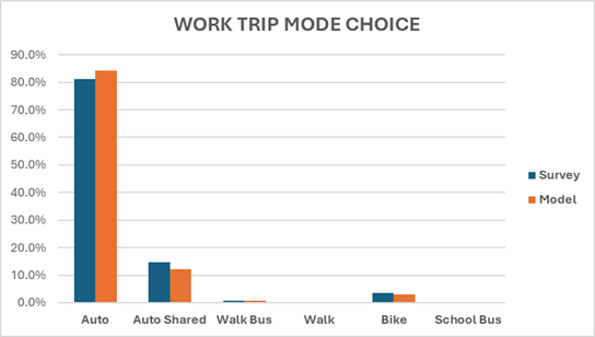
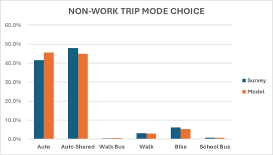
The mode choice model was validated against the available expanded survey data. These summaries are presented below.

Figure 13: Work Mode Choice Validation

Work

Observed		Estimated		Estimated Scaled		Observed %		Estimated %
Mode	Trips	Mode	Trips	Mode	Trips	Mode	Percent	Mode	Percent
Auto	181,419	Auto	200,962	Auto	200,962	Auto	81.2%	Auto	84.2%
Auto Shared	32,606	Auto Shared	28,857	Auto Shared	28,857	Auto Shared	14.6%	Auto Shared	12.1%
Walk Bus	1,574	Walk Bus	1,499	Walk Bus	1,499	Walk Bus	0.7%	Walk Bus	0.6%
Walk	140	Walk	217	Walk	217	Walk	0.1%	Walk	0.1%
Bike	7,684	Bike	7,213	Bike	7,213	Bike	3.4%	Bike	3.0%
School Bus	–	School Bus	–	School Bus	–	School Bus	0.0%	School Bus	0.0%
Total	233,424	Total	238,748	Total	238,748	Total	100%	Total	100%

Figure 14: Non-work Mode Choice Validation

Non-Work

Observed		Estimated		Estimated Scaled		Observed %		Estimated %
Mode	Trips	Mode	Trips	Mode	Trips	Mode	Percent	Mode	Percent
Auto	786,045	Auto	1,128,195	Auto	1,128,195	Auto	41.5%	Auto	45.6%
Auto Shared	908,111	Auto Shared	1,109,467	Auto Shared	1,109,467	Auto Shared	47.9%	Auto Shared	44.9%
Walk Bus	9,121	Walk Bus	12,699	Walk Bus	12,699	Walk Bus	0.5%	Walk Bus	0.5%
Walk	59,630	Walk	73,503	Walk	73,503	Walk	3.1%	Walk	3.0%
Bike	115,794	Bike	131,939	Bike	131,939	Bike	6.1%	Bike	5.3%
School Bus	15,377	School Bus	16,677	School Bus	16,677	School Bus	0.8%	School Bus	0.7%
Total	1,894,078	Total	2,472,480	Total	2,472,480	Total	100%	Total	100%

3.3 Time of Day Calculation

Time of day calculation: The time-of-day distribution of trips in the aggregate tour-based structure is based on direct application of empirical departure time profiles of each activity pair by person type. These departure time profiles were extracted from the existing travel survey. Since the travel survey was from 2010, it did not account for the post-covid changes seen in the time-of-day distribution of travel. An updated travel survey or other alternative information would allow a more accurate modeling of time-of-day travel patterns. A more detailed discussion around this issue presented in the later section on simulation-based dynamic assignment (SBA).

3.4 Network Assignment

Network assignment: Only motorized modes are assigned to obtained network flows in the PPACG model. Traffic assignment is performed for five macro time periods: Early, AM, MD, PM and Evening. Network flows from each of the time periods are aggregated into daily traffic flows. Headway based assignment is used for transit assignment. Demand is calculated at the same resolution as the traffic

assignment and assigned at once with AM, PM periods using an average peak headway and the Early, MD and Evening periods using an average off-peak headway.

Traffic Assignment Validation

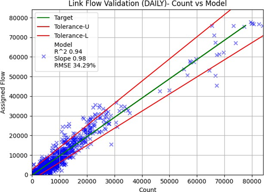
The traffic assignment was validated using the AADT model flows and average traffic counts available. An RMSE of 35%, R² of 0.94 and slope of 0.98 was achieved for the overall network. The statistics for each major link classification are presented in the table below.

FACTYPE	FACNAME	NUMOBS	SLOPE	%RMSE
1	Interstates	32	0.939	8.10%
2	Expressway	49	1.016	14.80%
3	Principal Arterials	375	1.24	23.80%
4	Minor Arterials	285	0.815	37.10%
5	Collector	312	0.772	59.90%
6	Residential	0	0	N/A
7	Ramp	93	1.007	28.30%

Transit Assignment Validation

The transit assignment was validated against overall line boardings. The mode choice coefficients were adjusted to produce overall line boardings that reflected the overall observed line boardings. The transit system has seen a steady decline in ridership from 2019 to 2021. As a result, an average of total line boardings over this period was used to validate the transit line boardings produced by the model. The transit route choice was not specifically calibrated due to the overall sparsity of ridership and relatively older travel survey. The boardings by route are summarized in the table below.

ROUTE_ID	ROUTE_CODE	ROUTE_NAME	MODEL_BOARDINGS	OBS_BOARDINGS
1	MMT_3416	Hillside – Hancock Plaza	555	564
10	MMT_3417	Hwy 115 – PPSC	218	425
11	MMT_3418	World Arena – PPSC	459	670
12	MMT_3419	Palmer Park Blvd	139	73
14	MMT_3420	Chestnut St – G.O.G. Rd	99	179
15	MMT_3421	Fountain Blvd – E Cheyenne Mtn Blvd	44	52
16	MMT_3422	Brookside – Uintah Gardens	112	85
17	MMT_3423	19th Street / Fillmore	79	68
18	MMT_3424	Union Blvd	105	20
19	MMT_3425	Weber – Eagle Rock	131	263
2	MMT_3426	Centennial Blvd – G.O.G. Rd	76	119
22	MMT_3427	Southborough via Murray Blvd	322	218
23	MMT_3428	Barnes Rd. – Tutt Blvd	421	258
25	MMT_3430	N. Academy Blvd – Voyager	1,556	802
27	MMT_3431	S. Academy Blvd – PPSC	477	458
3	MMT_3432	Colorado Ave – Manitou	341	534
32	MMT_3433	Security / Widefield	189	88
33	MMT_3434	Incline / Cog Shuttle	32	400
34	MMT_3435	G.O.G. / Austin Bluffs Pkwy	158	123
35	MMT_3436	Las Vegas St / PPSC	28	47
38	MMT_3439	Union / Childrens Hospital	64	7
39	MMT_3440	Corporate Dr – Voyager Pkwy	123	54
4	MMT_3441	S. 8th Street – Broadmoor	155	202
40	MMT_3442	Voyager – Rampart PPSC	51	32
5	MMT_3443	Boulder – Citadel	744	923
6	MMT_3444	Fillmore – Citadel	137	131
7	MMT_3445	Pikes Peak Ave. – Citadel	235	355
8	MMT_3446	Cache La Poudre – Citadel	32	67
9	MMT_3447	Nevada – UCCS	237	344
ZEB	MMT_3448	ZEB Downtown Shuttle	438	65
TOTAL			7,757	7,626

3.5 Simulation Based Dynamic Traffic Assignment (SBA)

One of the key uses of the PPACG model is evaluation of air quality conformity and GHG analysis. While the actual GHG analysis is performed using US EPA’s MOVES software, the link speed and volume inputs required in the analysis are generated using the PPACG model. The link speed and volume inputs are required at hourly intervals. As a result, simulation based dynamic traffic assignment (SBA) integrated into Visum was used as a post-process to obtain network link speeds at hourly intervals with relevant accounting of intersection level delays. SBA involves two components. Network preparation and hourly demand generation. These two items are discussed next.

Network Preparation for SBA

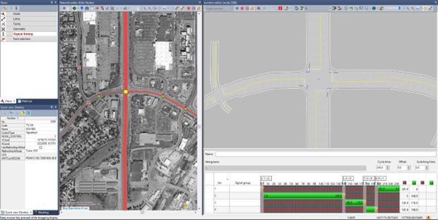
The Visum modeling platform used to implement the PPACG model natively stores multi-resolution network data. Here, the detailed lane geometry and intersection control (signal timings) can be specified in addition to the typical link-node data used in static traffic assignments. The appropriate level of network detail is used or ignored based on the type of traffic assignment selected by the user. The multi-resolution network storage concept is illustrated in the figure below.

The entire PPACG model network was carefully reviewed for the correct number of roadway lanes, posted speeds and intersection control type. Aerial imagery was used to code detailed intersection geometry with appropriate turn bays and lane grouping at all intersections in the model network. The network base year for the model is 2020. There are ~1500 controlled intersections in the model network. Out of these, ~700 intersections are signalized. Signal phasing plans for all these intersections were developed based on the lane grouping at approach legs. The green time and splits were calculated based on turn flows obtained from the static traffic assignment. Coding signal timings in this manner allows an overall consistent delay representation in the network. It also allows the methodology to be extended to all forecast networks.

Figure 15: Integrated Multi-resolution Network Representation in Visum

Demand Preparation for SBA

The tour-based model allows flexibility in specifying outputs for any time of day. Ordinarily, the hourly demand for the SBA would be derived by specifying an hourly demand output setting in the tour-based model calculation setup.

Figure 16: Pre-COVID19 Demand Profile vs Post-COVID19 Count Profile

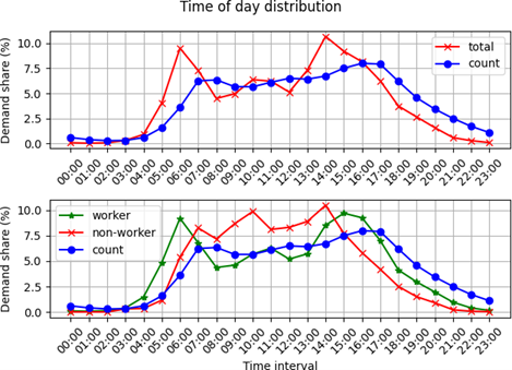
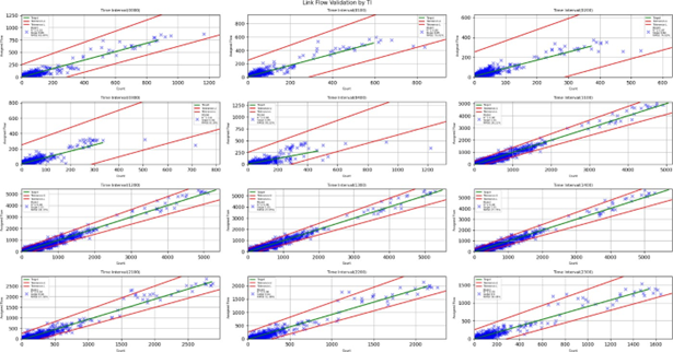
However, the changes in time use patterns seen after COVID19 and time of day factors derived from relatively older travel survey data (2010) made the direct use of time-of-day factors applied to activity pairs unviable. This was clearly seen by plotting the 24-hour demand profiles from the travel survey against the more updated 24-hour count data. The post-COVID19 time-of-day count profiles exhibit a much greater spreading of the traffic flows as opposed to the shaper AM and PM peak flows exhibited by the demand profiles extracted from the pre-COVID19 2010 travel survey. This change in travel pattern presented a major challenge in the development of 24-hour demand profiles and model calibration in general. Since count data was the most updated source of time-of-day distribution of traffic patterns, dynamic matrix estimation was used to re-profile the demand calculated for macro time periods (EA, AM, MD, EV) into hourly trip tables for use in SBA. The link flow validation for hourly flows is tabulated and plotted below. The early morning and late evening time periods have a greater %RMSE due to the overall lower volumes but are within the NCHRP allowable tolerance for hourly flows.

Table 13: SBA Hourly Link Flow Validation

Time Interval	R2	Slope	%RMSE
00:00	0.93	0.86	63.64%
01:00	0.89	0.85	75.01%
02:00	0.87	0.82	74.52%
03:00	0.8	0.82	81.80%
04:00	0.66	0.59	99.22%
05:00	0.76	0.78	72.51%
06:00	0.89	0.91	42.61%
07:00	0.93	0.98	32.52%
08:00	0.95	0.98	31.37%
09:00	0.96	0.98	30.18%
10:00	0.96	0.99	28.19%
11:00	0.96	1.01	28.21%
12:00	0.96	1.01	28.15%
13:00	0.96	1.01	27.65%
14:00	0.96	1.01	27.75%
15:00	0.95	1.02	29.80%
16:00	0.95	1.02	29.45%
17:00	0.95	1.01	29.61%
18:00	0.95	0.99	32.55%
19:00	0.94	0.98	42.88%
20:00	0.93	0.99	47.45%
21:00	0.94	0.96	47.56%
22:00	0.94	0.93	51.48%
23:00	0.93	0.90	58.48%
DAILY	0.96	1.00	27.78%

Figure 17: AM Period Hourly Link Flow Validation

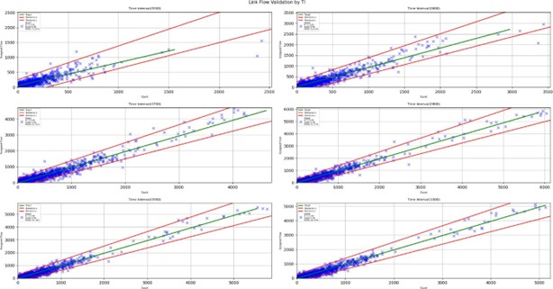
Figure 18: PM Period Link Flow Validation

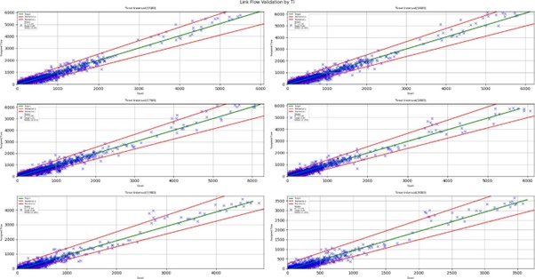
Figure 19: OP Link Flow Validation

The dynamic matrix estimation method implemented in Visum is based on a least squares minimization formulation. Here, the sum of squared error between network counts and network flows arising from traffic assignment is minimized using a gradient method.

Conceptually, the dynamic matrix estimation method is like the static variant but adds a time dimension to the problem formulation. In the dynamic variant, the rows of the flow matrix no longer correspond to the count locations, but to the cross product of count locations and analysis time intervals; the columns of the flow matrix no longer correspond to the quantity of the OD pairs, but to the entire demand time series. An entry in the flow matrix corresponds to the proportion of the demand of an OD pair during a demand time interval that passes a count location during an analysis time interval.

Since the original seed trip matrices and total number of trips are used in the overall solution formulation, the method also minimizes the distortion of the original matrix structure and preserves the number of trips in the seed matrices. This property also allows the use of adjusted base year hourly trip matrices to generate hourly link flows when assigned using SBA and as a reasonable basis for generating hourly trip matrices for the forecast years. As noted earlier, re-calibration of the tour-based model based on more steady traffic patterns and an updated travel survey would eliminate the necessity of using the dynamic matrix estimation post-process to obtain hourly trip matrices aligned with the observed time of day traffic patterns.

Figure 20: Steps to Obtain Hourly Link Flows – Base Condition

The methodology used in developing hourly trip assignment matrices for the forecast conditions is illustrated in the flowchart below.

4. Remarks

One of the challenges in the model calibration process was that the available travel survey was from 2010, and the latest data used in the model validation was over multiple years starting 2019 and ending 2022 with the COVID19 pandemic and its effects occurring during this period. As a general strategy, the model was thus not overfit to observations. It would be of benefit to take up a more thorough calibration and validation exercise when new travel survey data with a more stable set of observations from new travel trends is available.